Gene Imputation (3D)

Note

The 3D Gene Imputation is computationally intensive and may require several hours to complete, depending on dataset size and hardware configuration.

!git clone https://github.com/lanshui98/UniST.git
%cd UniST
!pip install -r requirements.txt

Note that the spatial information should be at adata.obsm['spatial'].

Put the adata under external/SUICA_pro/data/.

%cd external/SUICA_pro

Read the Data

!pip install scanpy
import scanpy as sc

adata = sc.read('data/3D_data.h5ad')
genes = adata.var_names

Example: get the index of gene “Myl2”

gene_idx = genes.get_loc("Myl2")
print(gene_idx)

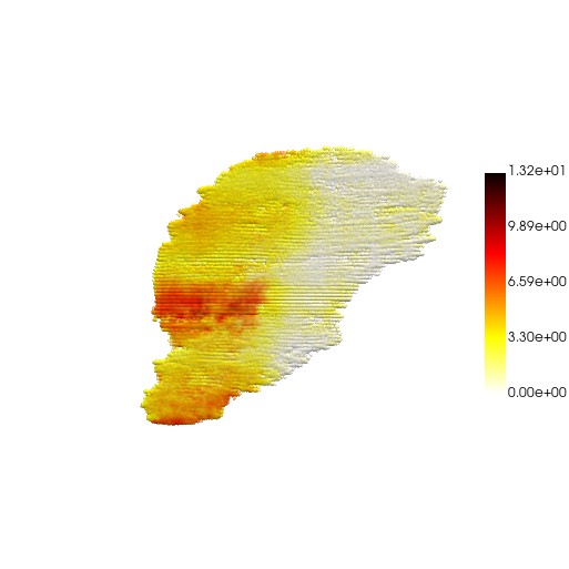
Visualization

from unist.downstream.vis import construct_pc, three_d_plot

# if you encounter: initialized module 'pyvista' has no attribute '_plot', try this:
!python scripts/patch_pyvista_circular_import.py

adata.obs["Myl2"] = adata.X[:,gene_idx].toarray().copy()

pc, cmap = construct_pc(
    adata=adata,
    spatial_key="spatial",
    groupby="Myl2",
    colormap="hot_r"
)

three_d_plot(
    model=pc,
    key="Myl2",
    colormap="hot_r",
    model_style="points",
    model_size=4.0,
    show_legend=True,
    jupyter="trame",
    legend_loc="center right",
    opacity=0.5
)

• "static" for static image

• "trame" for interactive window (need to install nest_asyncio2)

For more 3D visualization/animation details, please go to Animation.

---

Step1: Train GAE

! python train.py --mode embedder --conf ./configs/ST/embedder_gae_3d_sparse.yaml

Visualize the embeddings

emb = sc.read('logs/GAE-3D-sparse/3d_sparse/lightning_logs/version_0/embedded-all.h5ad')
emb.obs["emb1"] = emb.obsm["embeddings"][:, 0]

pc, cmap = construct_pc(
    adata=emb,
    spatial_key="spatial",
    groupby="emb1", 
    colormap="viridis_r",
)

three_d_plot(
    model=pc,
    key="emb1",              
    colormap="viridis_r",        
    model_style="points",
    model_size=4.0,
    show_legend=True,
    jupyter="trame",
    legend_loc="center right",
    opacity=0.5
)

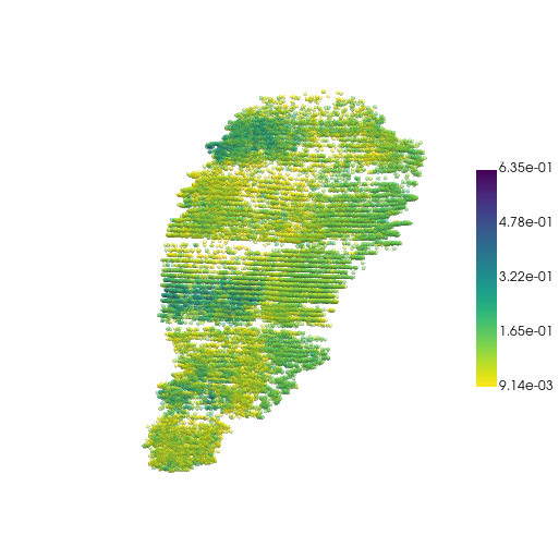
Notice how the z-axis is amplified here.

Certain parameters are set to handle sparse z-direction in 3D spatial transcriptomics data (e.g., when slice spacing is large).

use_anisotropic_knn: True

• Meaning: Whether to use anisotropic KNN graph construction

z_weight: 2.0

• Meaning: Weight factor for z-direction

• Effect:

  • > 1: Reduces the influence of z-direction distance

  • Calculation: weighted_z = z / z_weight

  • For example, z_weight=2.0 means z-direction distance is halved, making z-direction points more likely to become neighbors

• Principle:

  Original distance: d = sqrt((x1-x2)² + (y1-y2)² + (z1-z2)²)
  Weighted:          d = sqrt((x1-x2)² + (y1-y2)² + (z1-z2)²/z_weight²)
  

z_threshold: null

• Meaning: Maximum connection distance threshold in z-direction

• Effect:

  • null/None: Automatically set to 30% of z-direction range

  • Numeric value: Manually set maximum z-distance (in original coordinate units)

• Principle:

  • Even after weighting, if two points are too far apart in z-direction, they should not be connected

• Example:

  # If z_range = 1000 (from z=0 to z=1000)
  # z_threshold = null → automatically set to 1000 * 0.3 = 300
  # This means points with z-direction distance > 300 will not be connected
  

preserve_z_scale: True

• Effect:

  • True: z-direction is not compressed, maintaining a relatively larger range

  • False: z-direction is compressed together with xy-directions to the same range

• Principle:

  # preserve_z_scale = False
  # All directions compressed to [-1, 1], maintaining aspect ratio
  scale_x = x_range / max(x_range, y_range, z_range)
  scale_y = y_range / max(x_range, y_range, z_range)
  scale_z = z_range / max(x_range, y_range, z_range)
  
  # preserve_z_scale = True
  # z-direction maintains larger range, not compressed
  scale_x = x_range / max(x_range, y_range)
  scale_y = y_range / max(x_range, y_range)
  scale_z = z_scale_factor
  

z_scale_factor: 1.5

• Meaning: Scaling factor for z-direction (only effective when preserve_z_scale=True)

• Effect:

  • = 1.0: z-direction maintains original relative scale

  • > 1.0: Amplifies z-direction importance (recommended for sparse z-direction)

• Principle:

  normalized_z = (z - z_min) / z_range  # Normalize to [0,1]
  normalized_z = (normalized_z - 0.5) * 2.0  # Transform to [-1,1]
  normalized_z = normalized_z * z_scale_factor  # Apply scaling factor
  

Step2: Train INR + fine-tune GAE

! python train.py --mode inr --conf ./configs/ST/inr_embd_3d_sparse.yaml

Fourier Feature Encoding Parameters for sparse z-direction:

encoding_scales: [1, 10, 100]

• Meaning: Multi-scale frequency bands for Fourier feature encoding

• Effect:

  • Each scale creates a separate frequency encoding

  • [1, 10, 100] means three frequency bands: low (1), medium (10), and high (100)

  • Higher scales capture finer details, lower scales capture global patterns

• Principle:

  For each scale s in [1, 10, 100]:
    - Generate random matrix B with scale s
    - Encode: sin(2π * x @ B), cos(2π * x @ B)
    - Concatenate all encodings
  

• Why multiple scales?

  • Single scale can only capture one frequency range

  • Multi-scale captures both global (scale=1) and local (scale=100) patterns

  • Better representation for complex spatial structures

anisotropic_3d: True

• Meaning: Use different frequency encodings for xy-directions and z-direction

• Effect:

  • True: xy-directions and z-direction are encoded separately with different frequencies

  • False: All directions use the same encoding frequencies

• Why needed?

  • z-direction is sparse (large slice spacing)

  • z-direction needs lower frequencies to capture slice-level patterns

  • xy-directions need higher frequencies to capture within-slice details

• Implementation (see external/SUICA_pro/networks/ffn.py, lines 68-83):

  if anisotropic_3d:
      # xy-direction encoding (first 2 dimensions)
      xy_encodings = [GaussianEncoding(2, mapping_size, scale=s) 
                      for s in encoding_scales]  # [1, 10, 100]
      
      # z-direction encoding (3rd dimension)  
      z_encodings = [GaussianEncoding(1, mapping_size, scale=s)
                     for s in z_scales]  # [0.1, 1.0, 10.0]
  

z_scales: [0.1, 1.0, 10.0]

• Meaning: Frequency scales specifically for z-direction encoding

• Effect:

  • Only used when anisotropic_3d=True

  • z-direction uses these scales instead of encoding_scales

  • Typically lower than xy-direction scales (because z is sparse)

• Comparison with encoding_scales:

  xy-direction: encoding_scales = [1, 10, 100]     (higher frequencies)
  z-direction:  z_scales = [0.1, 1.0, 10.0]        (lower frequencies)
  
  Ratio: z_scales are approximately 10x lower than encoding_scales
  → z-direction uses 10x lower frequencies
  → Captures slice-level patterns, not fine z-direction details
  

• Why lower frequencies for z?

  • z-direction is sparse: large distances between slices

  • High frequencies would create noise between distant slices

  • Low frequencies capture smooth variations across slices

Step3: Prediction/Imputation

Prepare normalized custom coords

! python prepare_custom_coords.py --mode 3d --reference data/3D_data.h5ad --coords data/3D_coords.xyz --output data/preprocessed_data/custom_coords_3d_norm.npy --keep_ratio True --preserve_z_scale True --z_scale_factor 1.5

Run prediction

! python predict.py --mode inr --conf ./configs/ST/inr_pred_3d_sparse.yaml       

Map reconstructed coords back to original space

! python map_coords_back.py --reconstructed reconstructed-custom-3d.h5ad --reference data/3D_data.h5ad --output reconstructed-original-3d.h5ad --mode 3d --keep_ratio True --preserve_z_scale True --z_scale_factor 1.5

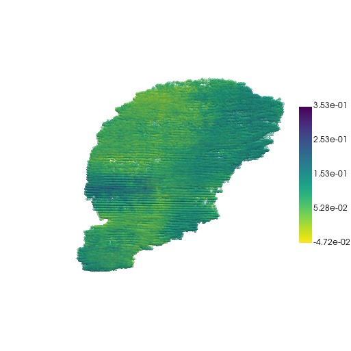
Visualize the fitted embeddings

res = sc.read("logs/GAE+FFN-3D-sparse/3d_sparse/lightning_logs/version_1/reconstructed-original-3d.h5ad")
res.obs["emb1"] = res.obsm["fitted_embd"][:, 0]
res.obs["emb1"] = res.obsm["fitted_embd"][:, 0].toarray().flatten()

pc, cmap = construct_pc(
    adata=res,
    spatial_key="spatial",
    groupby="emb1", 
    colormap="viridis_r",
)

three_d_plot(
    model=pc,
    key="emb1",              
    colormap="viridis_r",        
    model_style="points",
    model_size=4.0,
    show_legend=True,
    jupyter="trame",
    legend_loc="center right",
    opacity=0.5
)

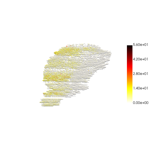
Visualize the result

res.obs["gene1"] = res.obsm["reconstructed_raw"][:, 0]

pc, cmap = construct_pc(
    adata=res,
    spatial_key="spatial",
    groupby="gene1", 
    colormap="hot_r",
)

three_d_plot(
    model=pc,
    key="gene1",              
    colormap="hot_r",        
    model_style="points",
    model_size=4.0,
    show_legend=True,
    jupyter="trame",
    legend_loc="center right",
    opacity=0.5
)